Basic Types, shapes, Grid and Geometry Mesh used in CFD

Basics of Meshing in CFD

Discretizing a domain into small elements or cells is known as meshing. Meshing is a very important part of numerical analysis. If the number of cells in a meshed domain are high the accuracy of analysis will be greater. Mesh is kept fine in the areas where capturing the physics of phenomenon is important. Mesh independence is one of the most important step in meshing. Mesh Independence is achieved by refining the mesh till the value of required variable becomes constant. Mesh refining requires high computational capabilities. Mesh can be classified into different types based on the uniformity and shape. Definitions of some elementary terms of meshing are given below (D. J. 1996).

Node: Point where two or more edges meet.

Edge: Boundary of a face

Face: Boundary of a cell

Cell: Control volume into which the domain is discretized.

Zone: Grouping of nodes faces and cells

Material data and source terms are assigned to cell zone whereas boundary conditions are applied on face zones.

Order of Meshing:

Mesh is generated in the order given below.

• Edge mesh

• Boundary mesh

• Face mesh

• Volume mesh

Mesh Independence:

Mesh independence is performed to see whether the size of mesh affects the solution or not. In this process, an initial mesh is generated and results are analysed for the conversion. If the conversion is not achieved, mesh is regenerated and checked to accomplish convergence. When the solution converges, mesh is refined (No of cells or elements are increased) to obtain better results. A residual limit can be set based on the problem to check for the error. With each refinement, results are obtained and compared to the results obtained with the previous mesh. If the results of two consecutive meshes are not same, mesh is refined again and again till the results become same. When the results for the two consecutive refinements are same, the previous mesh is believed to be generating accurate results.

TYPES of Meshing Based on Cell shape and Dimension:

A mesh can be two or three dimensional (D. J. 1996)

1) Two Dimensional Mesh:

            Two dimensional mesh can comprise of triangular or quadrilateral elements.

Triangular mesh:

In this type of mesh, cells are of triangular shape. Comparatively a very small amount of effort and time is usually required to generate this type of mesh. Triangular mesh is usually used in the domain areas where the physics of the problem is not very important.             

Quadrilateral Mesh:

In this type of mesh, cells are in rectangular shape. This shape is common in two dimensional structured mesh.             

 

Figure 9 types of 2D mesh

2) Three Dimension

In three dimensional meshing, a cell can have a shape of quadrilateral pyramid, tetrahedron, hexahedron or triangular prism. All of them have quadrilateral and triangular faces.               

Two dimensional extruded models can be represented completely by the hexahedron and prisms as extruded quadrilaterals and triangles.

In three dimensional meshing, quadrilateral faces might not be impeccably planar. A thin tetrahedron which is shared by two elements can be thought of a non-planar quadrilateral face.

Tetrahedron:

In geometry, a tetrahedron also known as a triangular pyramid, consists of four triangular faces, four vertices, four sides and six edges. This form of mesh can be auto-generated

Pyramid

This shape have four triangular faces, one quadrilateral face, eight edges and five vertices. They are utilized as transition elements between triangular and square elements. They are also used in hybrid grids.

Triangular prism:

This type of cell have six vertices and nine edges bounded by three quadrilateral faces and two triangular faces. It is very effective in resolving boundary layer.

Hexahedron

This type of cell have eight vertices and twelve edges bounded by six quadrilateral faces. Hexahedron mesh is considered best among all and it give the solution with highest accuracy. 

The triangular prism and pyramid zones can be considered computationally as degenerate hexahedrons, wherein some edges were decreased to 0. Other degenerate sorts of a hexahedron may also be represented.

Advanced Cells (Polyhedron)

It is a three dimensional element which can have any number of edges, faces and vertices. Large number of calculations are performed due to large number of neighbouring cells. This mesh is created to obtain more accuracy in calculations.

Figure 10 types of mesh

Uniform and Non Uniform Meshing:

In a uniform mesh, shape of cells throughout the domain is same whereas non-uniform mesh uses a blend of different mesh shapes. All the numerical approaches are designed to produce as small amount of errors as possible. These errors arises due to non-linear behaviour of the solution and large gradients of the physical properties in some places of the domain. This means that we need to handle small large-scale physical phenomena at the same time and these different phenomena can have a strong coupling with each other (D. J. 1996).

Grids:

The grid labels the elements or cells on which the flow is being solved.

• Represent the domain in a discrete manner

• Elements are grouped into boundary zones where boundary conditions has to be applied. 

• The mesh affects the rate of convergence, computational time and accuracy of the solution.

• Following parameters of the mesh are very important to obtain an accurate solution i.e. adjacent cellular extent/duration ratios, grid density, Tetrahedral vs. Hexahedral, skewness, mesh refinement thru adaption and Boundary/Inflation layer mesh.

Structured grids:

A structural grid spreads over a domain in a regular manner. In two dimensional meshing, structural grids have quadrilateral elements whereas in three dimensional structural meshing the elements are of hexahedron type. Structural gird is extremely space efficient. They display better solution convergence and generate accurate numerical results.

Unstructured grids:

Unstructured grids spread over a domain in an irregular manner. This type of mesh can be generated using any type of elements. The values at the nodes of unstructured mesh are very difficult to be represented in two or three dimensional arrays. Comparatively, an unstructured mesh is less space efficient. In two dimensional unstructured mesh, triangular shaped elements are used whereas in three dimensional unstructured mesh the elements are of tetrahedral shape

Figure 11  structured and non-structured Grid

Hybrid grids:

A hybrid mesh have both structured and unstructured mesh patches spread over the entire domain in a well-organized way. In the hybrid mode of meshing, structured grid is generated in the plain areas while unstructured meshing is generated in the areas where geometry is complex

CFD analysis of Tesla Turbine

CFD Studies of Tesla Turbine

In Jung (2014) work the flow rate was chosen as 0.0001. Iteration of disc outer radius and fluid angular velocity was done to find the volumetric flow rate for single disc spacing. In order to obtain the overall volumetric flow rate, the disk configuration was multiplied by the overall number of discs, giving appropriate efficiency and torque values. There was an iteration of head and flow speeds. Via the nozzle, fluid makes its way and is guided between the discs. The fluid hits the disc at an inclination nearly tangentially to the outside of the rotor, locating the jet's absolute and radial velocity. It measured the torque and generated power.

Jung (2014) worked on a CFD model of a Tesla turbine based on the design parameters mentioned above. In Solidworks2013, 2 domains were formed. The revolving domain comprised of a rotor assembly and the stationary domain composed of a simplistic nozzle in the outer casing. Figure below illustrates the layout of two domains.

 

Figure 3 Tesla Turbine CAD model for CFD

In Jung (2014) work fluid parameters are provided to illustrate the contact of the disc with water. The value of the dimensionless structure constant R was found to be -0.042, which implies reasonable model precision and important viscous effects. The performance of the streamlined nozzle was 77.7%. The velocity streamlines and pressure gradient are seen in Figures below:

 

Figure 4 Velocity Streamline of Tesla Turbine

 

Figure 5: Pressure gradient of Tesla Turbine

Lampart (2011) employed a CFD tool to observe the dependency of different operating parameters on the total sum of injecting nozzles. Nitrogen was the working fluid used in Organic Rankine Cycle. Three sum of nozzles 2, 4 and 6 were used in the study. The nozzles were located along the perimeter of flow inlet and were at equal distance and are tilted at 10° from the tangent of the circumference.  The results of the study showed a good correlation between less number of nozzles and higher flow efficiency under different operating conditions. The indicative of relatively low power transfer efficiency and losses occurring under same flow entrance locations, yielded the shortest flow path of six nozzles turbine that happen inside the flow space that leads to relatively low power output as compared with the lesser amount of nozzles alongside turbine. For the off-design operating mass flow situations, the stimulated models show the increased efficiency of flow. This happens to be in agreement with the interpretation of better efficiencies being accomplished at smaller flow directions proposed by Rice et al. However, at low flow rates in the vicinity of 0 kg/s, the study could not achieve the functioning features of the friction-type micro turbine. Moreover, the characteristics of operation of the turbine as soon as flow approximates to 0 kg/s and established the efficiency to react 0 at such conditions explored by many other investigators including Harwood (2008). The contradictions are made on the research work of Rice and Crawford (1974) to keep increasing the turbine’s efficiency as the flow reaches the zero flow rate state.

A numerical approach is used to study the effect of two geometric parameters, the thickness of disc and distance between disc spacing, that influences the performance of Tesla multichannel turbines. Two types of turbines were under study; 1st was a one-to-one turbine and 2nd was a one-to-many turbine, to check the aerodynamic performance and flow behavior in terms of geometric variations. The outcomes show the reduction in isentropic efficiency of the one-to-one turbine to some extend while the one-to-many turbine becomes significantly inefficient. For instance, the turbine having a 0.5 mm distance between disk, the drop is below 7%, and afterward, the variations in the thickness of the disc from 1 mm to 2 mm, resulting in the drop of 45% to its actual value. The increment between the distance of disc spacing results in the variation in isentropic efficiency of both turbines in the manner of initial increment than decrement later on. An ideal value and higher range of efficacy exist to attain maximum isentropic efficiency and to maintain it at the upper level. The ideal distance of disc spacing in the one-to-one turbine is 0.5mm that is relatively lower than a one-to-many turbine having disc spacing of 1mm with a constant thickness of discs that is 1mm. The summary for designing a multichannel Tesla turbine is that the distance between disc spacing must be in the range of its higher efficiency level and the criteria for selecting the thickness of disc must be balanced on the parameters of aerodynamic performance and mechanical stresses. 

 

Figure 6 CFD analysis of tesla turbine

The flow pattern in the Tesla turbine is illustrated in the figure below, having an inlet flow rate of about 1.32 Kg/s and 0..6Kg/s respectively. It is concluded that by keeping the inlet flow rate constant, there is a reduction in rotational speed. The increase in width of the distribution region of high-speed fluid towards the outer rim of turbine discs also increases the region and capacity of liquid doing-work. There is high-speed fluid flow from the outer rim to the center when the inlet flow rate is larger. This results in a lowering of fluid capacity and region. That is the reason why the rotational speed must be low to enhance the efficiency of the Tesla turbine for converting energy. 

 

Figure 7 velocity and pressure distribution inside tesla turbine

A figure provided below shows the domain pressure of fluid having an inlet flow rate of 1.32Kg/s. The increment in domain pressure of the fluid is observed by increasing the radius of the disc. The maximum pressure at the inlet of the turbine always appears near the outer rim. The maximum pressure continuously increased by an increment in speed of rotation and there is an absolute fluctuation in the distribution of pressure at the outlet while the fluctuations in velocity are significant at a higher rotation speed. There are small variations in domain pressure distribution of fluid between several flow rates.

 

Figure 8 Pressure distribution inside tesla turbine

Study the flow of compressible fluids in a Pipe Lab Report

"Study the flow of compressible fluids”

Aim of this study is to understand the flow behavior compressible fluid when they are made to flow under different conditions like different initial velocity or flow inside pipe of different diameters

1. Understanding the flow of fluid

In order to study the flow of compressible fluids it is important to first understand the basic about the flow of fluid. 

This may include information about what fluid is, what are its types, what are different types of flow in which a fluid can flow.

2. Numerical analysis to predict the flow behaviour

Numerical analysis is done in engineering in order to predict the behavior of things when certain condition is applied on them. 

For this task this may include the computational fluid dynamics to predict the type of flow in fluid when it moves inside the pipe.

3. Experiment of air flowing through a pipe

An experiment will be performed to study the flow of air inside a pipe. Experiment will consist of three different pipes with difference in the diameter of pipe and many different initial velocities of the air entering the pipe. 

Experimental data will be collected and used for the calculation of Reynold number, friction factor and head losses inside pipe.

4. Compare the Numerical analysis and experimental data

In order to check the accuracy of the predicted flow behavior in numerical analysis a comparison will be made between numerical simulations and experimental results. 

Another comparison will also be made between calculated and graphical value of friction factor in order to check any variation in experimental data as compared to ideal values.

Fluid and Its Types

Fluid is any material that can flow from one point to another point due any reason or in the influence of any force. 

Fluid can be either in the form liquid or gas and in some gasses it can be converted from one form into another during flow. There two main types of fluids

1. Compressible fluid

Compressible fluids are those fluids which can undergo compression at molecular level when a certain amount of pressure is applied on them.

2. Incompressible fluid

Compressible fluids are those fluids which cannot undergo compression at molecular level when a certain amount of pressure is applied on them.

Types of Fluid flow

There three main types of fluid flow

1. Laminar flow

It is the type of flow where each proceeding particle follows the same path in the flow on which the first particle has moved during flow.

2. Transient flow

It this types of flow where each proceeding particle follows the same path with little disturbance in the flow on which the first particle has moved during flow

3. Turbulent

It is the type of flow in which each particle has its own path in flow and no one part follows the other particle in a stream.

Reynold Number

It is the ratio of fluid inertial forces to the fluid viscous forces. It’s a dimensional less quantity which is used to show the type of fluid flow. If the Reynold number of the fluid flow in less than 2100 then the flow is said to be laminar flow.

If the Reynold number of the fluid flow in greater than 2100 and less than 4000 then the flow is said to be transient and If the Reynold number of the fluid flow in greater than 4000 then the flow is said to be Turbulent flow.

Read about Open Channel Flow and Bernoulli Experiment

Computational Fluid Dynamics

Computational fluid dynamics is the branch of fluid mechanics which involve solving complex equations related to the fluid flow in in different conditions. 

Computational fluid dynamics is used to predict the behavior of fluid flow under the given condition. Computational fluid dynamics done in simulation program ansys consist of following steps

1. CAD modelling
CAD modelling is the process of making a computer added model of the required system using ansys workbench. 

In the current work pipe and fluid which is air will be modelled in this section and then assembled to make complete system

2. Meshing
Is this section the designed system is divided into very small sections call cells joined to each other through nodes or key points. 

This is done in order to get solution of governing equation for each section.

3. Setup
In this section the inlet, outlet and boundary walls of the system are setup along with the required values. In this section material properties of the system is defined. 

In this section the material properties of pipe like smoothness and fluid properties like density and fluidity are defined. 

Value of initial velocity is also defined in this section. For this work inlet velocity of 47.1 will be used with air a fluid and smooth pipe

4. Solution
In solution section type of solution is selected for the system and required output parameters are selected. 

When started solution section will calculated values of selected parameters and show them in the shape of colour figures. For this work transient type hybrids solution will be done.

Results

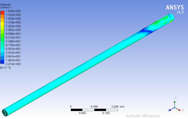
Based on setup made above simulation of the required system were run and result in terms of fluid velocity has been shown below.

According to the result flow of fluid inside the pipe will be turbulent as different velocities can be seen near inlet of the pipe along with the waves on entire length and especially on the top section of fluid domain.

It can be observed from the below mention figures that flow of fluid inside pipe is uniform and very smooth. This is due to the fact that wall roughness of the pipe is kept zero to make smooth pipe.

Experimental Results

Comparison

Moody chart mention below is used to find the frictional factor of the graphically and it is said to the ideal values of frictional factor as it does not consider the actual working conditions. 

For the initial velocity of 47.1 m/sec the experimental value of fractional factor is 0.0216 but for the calculated Reynold Number of 1*10^5 the graphical value is said to be 0.018 which quite less than the experimental value. 

The reason for high value of frictional factor in experiment is that pipe was considered smooth but it was not. Wall roughness of pipe add more value to frictional factor.

Discussion

The prediction made by the computational fluid dynamics for the behavior of the fluid flow is verified by the experimental data. 

Numerical analysis predicted that fluid flow will be turbulent in the pipe and according to the experimental results the calculated Reynold number for all initial velocities is above 4000 range which is for turbulent flow. 

This turbulent flow in smooth pipe is due to the high initial velocity as compared to the density of air.

According to the moody chart the frictional factor and Reynold number are connected to each other. So in order to find the relationship between these two a graph was generated which have friction factor on y axis and Reynold number on x axis. 

According to the trend shown in graph frictional factor and Reynold number are directly proportional to each other. Increase in value of Reynold number will increase the value of frictional factor and decrease in value of Reynold number will decrease the value of frictional factor

In order to find the relationship between mass flow rate and pressure drop a graph was generated which have pressure drop on y axis and mass flow rate on x axis. 

According to the trend shown in graph mass flow rate and pressure drop are directly proportional to each other. Increase in value of mass flow rate will increase the value of pressure drop and decrease in value of mass flow rate will decrease the value of pressure drop.

Flow of a Compressible Fluid Lab Report

Aim of this lab work is to understand the flow of a compressible fluid inside a tube

Following are some of the objectives which will lead to completion of above mention aim

1. Study the basic fluids, types of fluids and types of flow of fluid 

2. Perform the numerical analysis to predict the flow of fluid in smooth pipe 

3. Perform experiment of air flowing in smooth pipe

4. Calculate the Reynold number, friction factor and head losses in experiment

5. Compare the experimental result with calculated and numerical analysis

Introduction on Flow of a Compressible Fluid

Fluid is anything which can flow between points of high potential to the point of low potential is called fluid. Ability of the fluid to flow is called its fluidity of fluid and it depends on the viscosity of the fluid. 

Viscosity of the fluid is much like the density of the solid and it define the weight of the fluid per cubic meter. Higher the viscosity of fluid is higher will its weight per cubic meter and lower will be its fluidity. 

Fluids can be classified in many different types based on the things under discussion for example discussing the Newton law fluids can be classified as Newtonian fluid and Non-Newtonian fluid. 

Newtonian fluids are those fluids in which stresses at every point of flow are directly proportional and linear to strain and Non-Newtonian fluid are those fluids win which stresses at every point of flow are not directly proportional and linear to strain. 

Based on the ability to compress fluids can be classified as compressible and non-compressible fluids. 

Compressible fluid has the ability to get compress under high pressure means their particles just their position under pressure and non-compressible fluid are those fluid which does not show any change under pressure means their particle does not change their position under pressure. 

Learn Effect of Sluice Gate on the Flow of Fluid

Types of fluid flow

There are three main types of fluid flow and all of them are based on the Reynold number of that particular fluid flowing at any particular speed. Reynold number is a dimension less number which shows the fluid inertial forces as compared to the viscous forces. 

Based on the Reynold number fluid flow has three types; one is Laminar flow in which the Reynold number of the fluid never exceed 2100 value, transient flow is one in which Reynold number fluid flow lies between 2100 and 4000 value. Turbulent flow in one in which Reynold number of fluid flow exceeds 4000 value.

Numerical Analysis

In order to predict the flow of fluid in any condition numerical analysis of that condition is done. Numerical analysis is a theoretical solution or the answer of the question related to the flow of fluid.

Computational fluid mechanics is used to predict the flow of fluid in any required conditions and as this process is very complex computer software like ansys is used to solve the equations involve in this process. 

In order to perform the numerical analysis of this current process first the component involved in this work are needed to be modelled and for this any cad software or work bench of ansys can be used. 

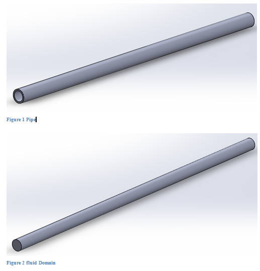
Figure one shown below is computer added model of pipe which represents the pipe used in this lab work. Second figure is of the fluid domain which represents the fluid which flow inside the pipe. Third figure represent the assembly of the pipe and fluid domain which will be used for analysis purpose. 

In ansys the all components are first named as required like pipe, fluid domain, inlet and outlets and then they are meshed. Inlet of the pipe is on the right side of the pipe and outlet is on the left side (face visible in below figures). 

In ansys setup the fluid domain is selected as fluid and air is selected as its material. For pipe material does not matter as long as analysis is limited to the flow of fluid. Pipe is made smooth by making the wall roughness zero in ansys setup. 

In solution section transient solution will be done in order to simulate the flow of fluid inside the pipe with the initial velocity of fluid entering the pipe is as per experiment requirement.

Result of the simulation shown above in figure 4 shows that at the inlet of the pipe the flow of fluid will be very turbulent as different velocities are visible in that region and along the length of the pipe the velocity on the top of the fluid domain and on the centre are different which shows fluid flow will be turbulent throughout the pipe.

Experimental Result
Table 1 Experimental value

The friction factor mention in the above table is called the experimental frictional factor or the actual frictional factor as the data provided for its calculation was generated by performing an experiment. 

Another way to get the friction factor is the moody chart which can predict the ideal friction factor based on the Reynold number and relative friction of surface. 

According the calculation made based on the experimental data the frictional factor for 34 mm diameter pipe and initial velocity of 51.4 meter per second is 0.021. 

According to the moody char for the Reynold number of 1.1*10^5 and smooth pipe the frictional factor is about 0.017 which is less than the experimental frictional factor. 
 

Figure 7 Moody Chart

Difference in the values of the experimental and graphs friction factor can be due to the fact that the pipe used in the experiment cannot be perfectly smooth that is the internal wall may have produce some extra frictional forces which result is additional pressure drop and increased value of frictional factor. 

Discussion on Flow of a Compressible Fluid

Numerical analysis of the said experiment was conducted using the computational fluid mechanics in ansys and result show that the flow of air inside the smooth pipe will be turbulent. 

According to the experimental results the calculated Reynold number of the flow for all conditions is above 4000 mark which shows that the flow of air inside the pipe for experimental setup was turbulent. 

So it can be concluded that the numerical analysis done for this experiment has successfully predicted the nature of flow of air inside the pipe.

In order observe the effect of mass flow rate on the change in pressure developed across the pipe, a graph was generated using the values obtain during the experiment. According to the graph the mass flow rate and change in pressure developed are directly proportional to each other. 

This means that the increase of mass flow rate of air inside the pipe increase the pressure difference observed across the pipe and decrease of mass flow rate of air inside the pipe decreases the pressure difference observed across the pipe

In order observe the effect of Reynold number on the frictional factor, a graph was generated using the values obtain during the experiment. According to the graph the Reynold number and frictional factor are directly proportional to each other. 

This means that the increase of Reynold number of air inside the pipe increase the frictional factor and decrease of Reynold Number of air inside the pipe decreases the Frictional factor for pipe with 24 mm and 16 mm diameter for 34 mm diameter this relation is opposite. 

Different Types of Fluid Flow Measurement Devices

Following are the different types of fluid flow measurement devices which are available for the flow rate measurement. 

• Orifice Plate
• Venture Tube
• Flow Nozzles
• Variable Area

Orifice Plate

Recommended: Orifice Plate Lab Report

Advantages of Orifice Plate

•Orifice plate is very simplest instrument available which is also very easy to install and remove

•Have high pressure recover efficiency of 65 percent

•Have the ability of measure flow rate over a wide rage

•Cost effective

Disadvantages of  Orifice Plate

•It only support those fluid that are homogeneous is nature

•It work under a limited viscosity of fluid

•Accuracy of orifice plate depends on fluid density, viscosity and pressure

•Working limited to horizontal applications

Venture meter 

Recommended: Venture Meter Lab Report

Advantages of Venture meter

• Offer horizontal, vertical and inclined flow measurement

• Perfect working behavior prediction

• Very high pressure recovery efficiency of 90 %

• Highly accurate for a wide range of flow rates

Disadvantages of Venture meter

•Required more space for installation as they have large is size due to their working method

•Have high initial cost 

•Difficult to install and remove

•Have limitation of minimum pipe diameter of 7.5 cm

Flow Nozzle

Advantages of Flow Nozzle

•Small in size as compared to venture meter

•Easy to install and remove

•Cost effective

•Discharge coefficient of flow nozzle is high

Disadvantages of Flow Nozzle

•Pressure recovery efficiency is low

•High maintenance cost

•Required more area as compared to orifice plate

Variable area

Advantages of Variable area

•Offers constant drop in pressure over the length of tube

•Simple construction

•Easy to install and maintain

•Work perfectly for liquid and gas

Disadvantage of Variable area

•Work only in vertical direction

•Transparent material is required for construction

•High pressure loss

•Limited rage for fluid viscosity

Four different types of flow measurement devices has been present above with their advantages and disadvantages and according to those venture meter is the best choice for the flow measurement devices, as it has highest value of pressure recovery efficiency, offer flow rate measurement in any direction and can work in wide range of flow rate. It has high cost and difficulty in installation but that’s one time cost for a flow measurement devices.